Model Selection and Prior Assignment

Related Content
carvalho09a.pdf
In my previous blog, I described the outline of the statistical process known as "the lasso" (Tibshirani 1996). The main aim of this method was to choose the covariates in the data which had the biggest impact on the response vector which we are aiming to study. To put this in more formal terms, the lasso allows us to select a set of covariates Xsβs which have a large affect on the results we are given. We are hence left with a set of unselected covariates Xuβu which we know have very little effect on the result of our experiment.
We now wish to use this new knowledge in order to make better inferences about the data which we have. There is however one problem with this thought. In order to formalise the theory of selecting such a model using the lasso, we want to know for sure which covariates (we shall call them S) are selected. However, as this is dependent wholly on the data, this selection could always be different, and hence is what we call a random process. This causes a problem, as normally this would mean we would first have to carry out a whole procedure of statistical analysis just to be able to say which model actually gets selected. Luckily however, there is a way we can avoid this by conditioning our whole experiment on the particular model chosen (This process was first championed by Tibshirani (2013)). We denote this choice of model as the event {S=s}, and in Lee et al. (2016) it was found that this event can instead be reformulated as an affine relation {AY ≤ b} (for more information on this, please have a look at my first blog here). When conditioning on this relation, we find that the distribution of our whole model (when we have used the lasso to select variables) is a truncated normal distribution, with the exact distribution shown below.
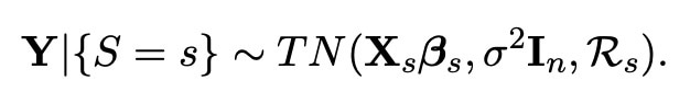 More information on what this phrase represents exactly can be found in Lee et al. (2016), but the important detail here is that ℜs is the region which can be found from the values which satisfy {AY ≤ b}. The reason we have written this distribution with the label "Y|{S=s}", is because this is how we write the likelihood of a variable when we are working in the Bayesian setting. A key part of the bayesian setting, is that we can assign each variable in our model a prior distribution depending on our knowledge and inference before the experiment has taken place. The bayesian setting is very useful in our investigation, as if we choose our priors correctly, it has been proven that bayesian methods actually outperform our usual statistical methods (known as frequentist methods) in terms of both accuracy and bias. What we wish to do here is therefore choose valid priors for each of our unknown variables.
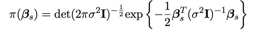
We start with the vector βs. As we know that these covariates were chosen by the lasso, we know that this vector contains most of the important information about the experiment. We hence know this data will act as we expect, and as we know that our likelihood function has a distribution which is normal (with truncation based on the selected covariates) we can choose our vector βs to have a normal distribution too. Specifically, we can assign the prior distribution below to this vector:
 We here choose the matrix Dκ to be the identity matrix I, so that calculations are easier and more efficient to carry out in our simulations. The probability density function for this normal distribution is also shown below.
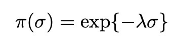
 We also assign the variance σ2 an exponential distribution, as is commonplace within bayesian statistics:
Normally, this information would be enough to perform a bayesian analysis and find important statistical results such as credible intervals. However, the main aim of my research is to improve these existing approaches. In order to do this, we need to incorporate some information about the unselected covariates Xuβu. The reason we do this is because whilst the lasso is a good selection tool, it is not perfect and may not select every variable of use. In fact, even if the lasso did select all of the useful variables in the model, it may still be useful to incorporate some of the left out information just in case there is a tiny affect on the experiment hidden within the data. We hence wish to assign a prior to the vector βu, so that any information from this vector can be included in our analysis. As we know that all of the elements of βu were not originally selected by the lasso, we know that their effects on the response vector Y must be quite small, with a lot of the covariates having no effect at all. We therefore call this data sparse, and there exists a prior known as the horseshoe prior (see Carvalho et al. 2008) which excels in sparse situations (as shown by Van Erp et al. 2018). The distribution of the horseshoe prior is shown below.
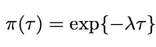
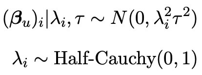 As we can see, this prior is quire complicated, and sadly it lacks the analytical form which makes many priors so easy to use. Thankfully however, we can use the Horseshoe package (created by Van Der Pas et al. 2019) in the programming language R to evaluate this prior. Here, we see that the prior distribution is also dependant on the variance parameter τ, and so we need to assign this a prior distribution too. As mentioned previously, we choose the common exponential prior for this distribution as detailed below.
Now, given this variance prior, we can use the horseshoe package in R to perform statistical approaches on this data. The horseshoe package is very useful, as not only does it allow for the prior to be assigned within the code, but it can also create important plots, find useful values and even create credible intervals (the bayesian version of a confidence interval) from the data we specify. One such plot is shown below, and plots the value of Xuβu on the y-axis against the response variable Y on the x-axis.
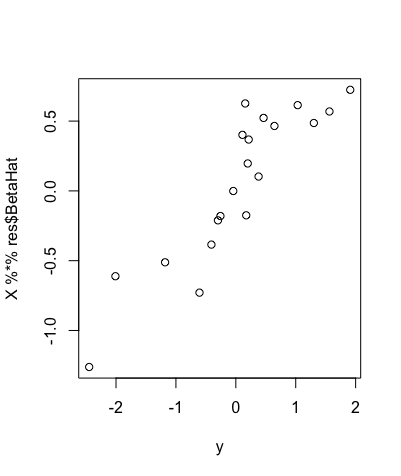
This is a useful plot, as it shows how the covariates we select affect the response variable Y directly. Furthermore, we can see in the plot above that if we were to draw a line of best fit through these data points, this line would be roughly straight, but there would be a lot of points away from this line, showing that these covariates do in fact affect the response variable Y in some way.
Another useful feature of the horseshoe package is that it allows us to find credible intervals. When using the same simulated data that gave the plot above, the code outputted the set of credible intervals shown below.
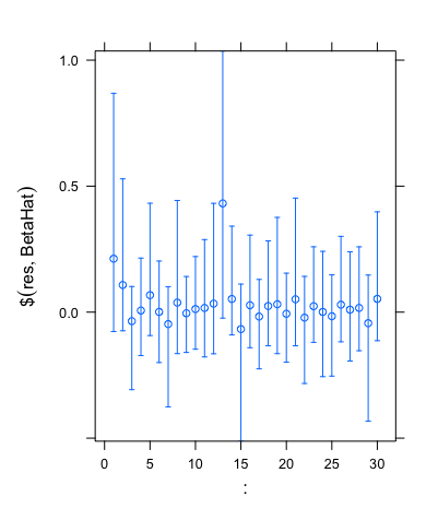
As we can see, these intervals are clear to read and analyse, and hence show how the horseshoe package can be used powerfully in practice.
Now we have all of the tools which we need to perform our desired bayesian analysis. We have a full set of prior distributions as given above, as well as a likelihood function. We can thus use the simple bayesian relation

to find the posterior distribution for our experiment. From this we can make our bayesian inferences and form credible intervals given a set of data which we wish to examine. This implementation will be the main focus of my research for the rest of my project, and hopefully this new method will display preferable performance and properties to methods which exist already in the world of high dimensional data.
References
Carvalho et al. 2008: Carvalho, C. M., Polson, N. G. and Scott, J. G. (2008). Handling Spar- sity via the Horseshoe. Journal of Machine Learning Research, W and CP 5 73– 80.
Tibshirani 1996: Tibshirani, R. (1996), ‘Regression shrinkage and selection via the lasso’, Journal of the Royal Statistical Society: Series B 58, 267–288.
Tibshirani 2013: Tibshirani, R. J. (2013), ‘The lasso problem and uniqueness’, Electronic Journal of Statistics 7, 1456–1490.
Van Erp et al. 2018: Van Erp, S., Mulder, J., and Oberski, D. L. (2018). Prior sensitivity analysis in default bayesian structural equation modeling. Psychological Methods, 23(2):363–388.
Van Der Pas et al. 2019: Van der Pas, Scott, J., Chakraborty, A., Bhattacharya, A. (2019). S., https://CRAN.R- project.org/package=horseshoe
I am a recent Mathematics Masters Graduate, having studied at Durham University. During my scholarship, I pursued a project detailing "valid post-selection inference" within the realm of statistics; with a particular emphasis on samples of large data sets, and developing new methods with which to evaluate such data. If you are interested in any of my work, or just want to make a new friend, please send me a message and I will be more than happy to help in any way I can.


Please sign in
If you are a registered user on Laidlaw Scholars Network, please sign in