Making inferences after model selection


Following on from my previous blog, we now have the correct form of the posterior distribution which best suits the setting described by high dimensional data. To summarise the work completed previously, we used a selection of appropriate prior distributions for each part of the model described by the data. These priors then gave way to form a posterior distribution which is found using a Markov Chain Monte Carlo (MCMC) method in the programming language R. The reason for using this MCMC method, is that given how the posterior has no specific analytic form to find, we needed to instead take samples from the given priors, and use them to simulate the posterior distribution. We repeat this process 6000 times, with the priors being updates with each iteration. These prior updates then converge towards the full posterior distribution, which we can then use to make the inferences which we desire.
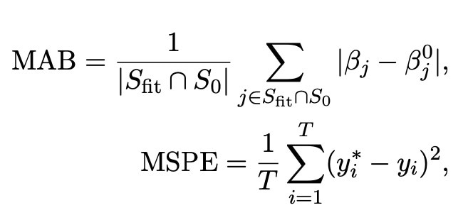
These inferences have been the main focus of my research over the past six weeks. By simulating the posterior distribution in the way described above, we are able to make a number of estimates which are not only useful for prediction purposes, but which are also statistically valid. The first of these estimates is that of the estimate of the selected covariates β*s. This is arguably the most important estimate, as this can be used to both estimate the values of the covariates which we select, as well as to predict future values from the data. We know how to find this estimate from the posterior, however we want to check that this estimate is actually useful and accurate. To do this, we first simulate a range of data under different settings. Within these simulations, we plant some covariates which we know are significant, and we note the values of these true covariates which we call βs0. We can then consider two key estimates: the mean absolute bias (MAB) and the mean squared prediction error (MSPE). The MAB estimates describe how far away the estimated covariates are from the true values, whereas the MSPE tells us how far any values predicted from the data are compared to the true values we know the simulated data will take. To describe things more mathematically, the two above estimates can be calculated as follows.
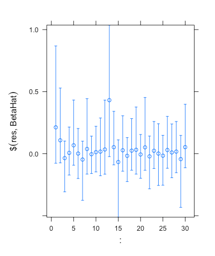
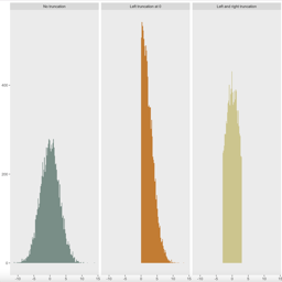
 The simulations which I have conducted provided such values. Many different conditions on the number of covariates, sample size and the number of true parameters were made, and an example of one of the results is shown in the image below. In order to show how my method worked in comparison with existing methods, I have also included the MAB estimates for the lasso (Tibshirani, 1996) and ridge regression: two key tools in high dimensional inference. These methods were conducted under the exact same simulation conditions as my method (denoted BE-PoS) in order to make sure the comparison is as fair as possible.
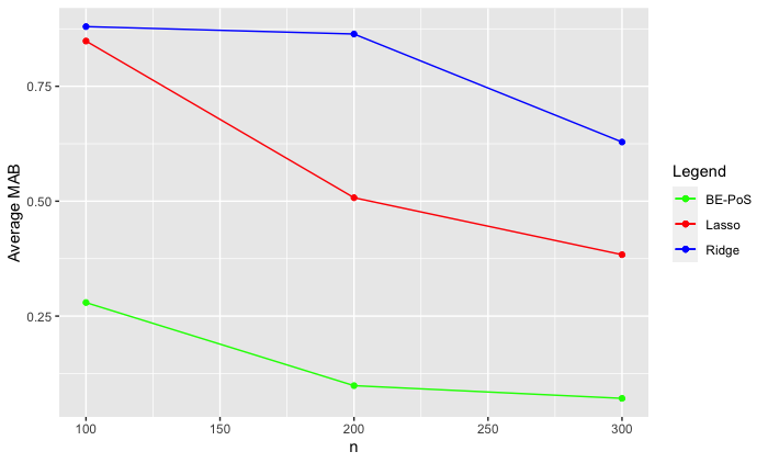 As we can see, the method which I have been working on has a much lower bias than the other two selected methods. Obviously this only describes one set of results, but a similar pattern was found in all of my simulations. This is an extremely useful property, as it represents how the new method outperforms existing methods in terms of estimation power.
Having established the strong estimation power of this new method, we also wish to examine the prediction power of the method. We hence compare the MSPE of the new method with existing methods under identical simulation settings. In order to be as thorough as possible, we compare the BE-PoS method with the lasso (Tibshirani, 1996) , ridge regression, the bootstrapped lasso (Chatterjee and Lahiri, 2011) and principle components regression (denoted PCR). the results are again shown in the image below.
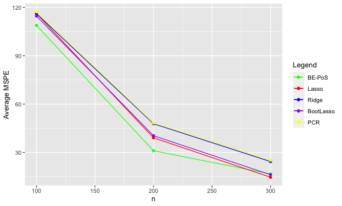 As we can again see, whilst not being as large a difference as shown in the MAB estimates, we see that the BE-PoS method again outperforms the existing methods in terms of prediction error.
The above two images and results serve to show how this new method is superior to existing methods in terms of prediction and estimation in the high-dimensional setting. There are however other important values to consider. One such value is that of a credible interval. A credible interval is useful, as it will represent a set of values which the true covariate values will lie between with a given probability. As a result of this informal definition, it is easy to see that is is better to have a shorter credible interval, as then we have a much better idea of exactly which value the true covariate takes. As a result, a key part of the simulations conducted involved examining the average length of the credible intervals in the model. The table below shows the results for a variety of different parameters (p), sparsity (s0) and observations (n).
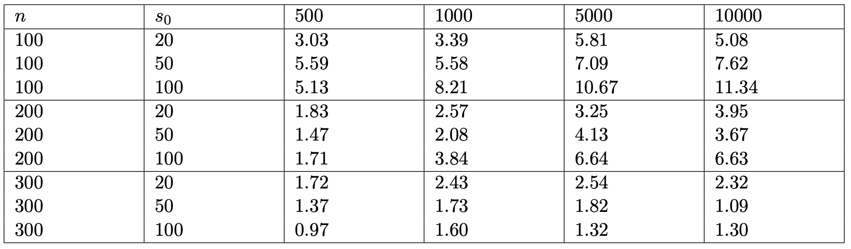 As we can see, when the number of parameters and sparsity are kept constant, the length of the credible intervals decreases towards zero. This is a very useful observation, as this implies that as the number of observations n tends towards infinity, the length of the credible intervals will converge towards zero. After some theoretical work, this is shown to be the case. The upshot of this is then that, if we were to observe enough information from an experiment, then we would have an incredibly short credible interval for where the true parameter lies. This would hence mean we have an extremely good idea of the true value of this covariate, which is a very useful property.
Overall, the culmination of my research over the past six weeks has culminated in the development of a new, statistically valid method with which to analyse high dimensional data. The review of past methods and Bayesian statistical methods has allowed for this method to be developed in a mathematically valid way, whilst the results from a range of simulations show how powerful this method is. The main takeaway from this research is the way in which it outperforms existing methods in this setting. Such a method is therefore both useful to provide new inferences about statistical problems in the world, as well as to form the basis of new methods which will further improve statistical ability within the high dimensional setting.
References
I am a recent Mathematics Masters Graduate, having studied at Durham University. During my scholarship, I pursued a project detailing "valid post-selection inference" within the realm of statistics; with a particular emphasis on samples of large data sets, and developing new methods with which to evaluate such data. If you are interested in any of my work, or just want to make a new friend, please send me a message and I will be more than happy to help in any way I can.
Please sign in
If you are a registered user on Laidlaw Scholars Network, please sign in