How To Predict The Future

Disclaimer: This article assumes no prior knowledge of physics or mathematics, apart from section VI which may be safely skipped.
I. Introduction
The staunch determinists among us would insist that the future is set in stone. This is precisely what the mathematician Pierre-Simon Laplace put forth with his thought experiment:
Suppose an intellect knew of the precise atomic history of the universe and the forces acting on every particle. Assuming that the intellect could analyse this vast ocean of data, it would see no distinction between the past, present, and the future.
Thankfully Laplace precedes all modern theories of quantum physics that inherently bring uncertainty to our computations. This is not a failure of the theory or a consequence of imprecise instruments. Uncertainty is woven into the very fabric of the model.
The essence of physics, much like any natural science, is to understand the why the world works the way it does. Given a current system, a physicist strives to uncover its future.
II. A bit about my research
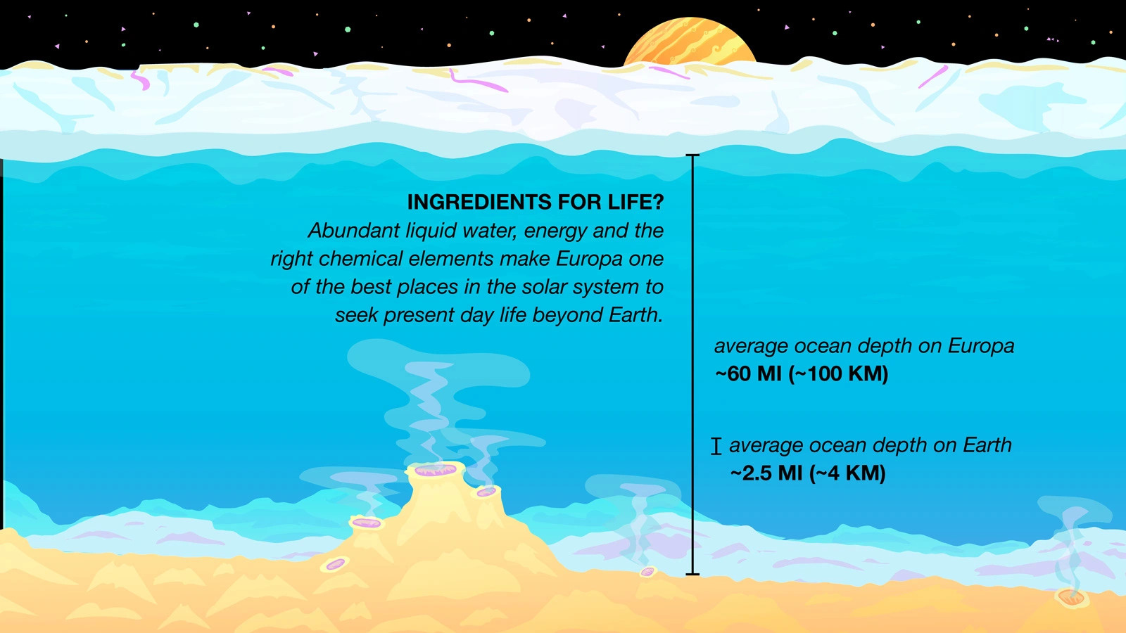
The potential of life existing beyond our little blue planet has been the subject of human fascination since the time of ancient Greece. We turn our attention to Jupiter and its moon Europa.
First discovered centuries ago by the legendary Galileo, contemporary analyses of Europa’s internal structure has rekindled much excitement in the scientific and science fiction communities. The reader may find it endlessly fascinating, much like I do, that Europa is wholly enveloped by a vast and deep ocean of water, capped at the surface by a thick layer of ice. Whether life exists in Europa depends on the nature of its oceanic currents and the consequential transport of salts. This brings us to the crux of my research: to measure the effect of thermal forcing (temperature) and sub-surface ice topology on the ocean’s currents.

To do this, the ice-ocean system must be modeled computationally such that I can explore the effect of different parameters on the system's evolution.
The most common question I recieve upon explaining my project is: how do you simulate this. This piece is dedicated to that question.
III. The essence of simulation
Every simulation, at its very foundation, follows the following algorithm.
- Analyse the state of the current of the system. This could be finding out the locations and speeds of all the particles in the system, and the forces acting on these particles. If we're just starting the simulation, we have to set these values ourselves.
- Use physical equations to calculate the state of the new system. This could be using Newton's equations to find out the new locations and speeds of every particle, a very tiny bit into the future.
- Repeat.
The computer scientists among us may realize that this is precisely the same algorithm used for coding games.
IV. A simple example
To demonstrate the principles of simulation, we design a new univerese. In this universe, there exists only an apple that may travel in a straight line. On this straight line there exists a centre point which we denote the origin. All distances are measured from this point. All points to the right of the origin have positive distance, while all points to the left of the origin have negative distance.
There exists no laws of physics in this universe but the following: the velocity of the apple at any position is equal in value to its distance from the origin.
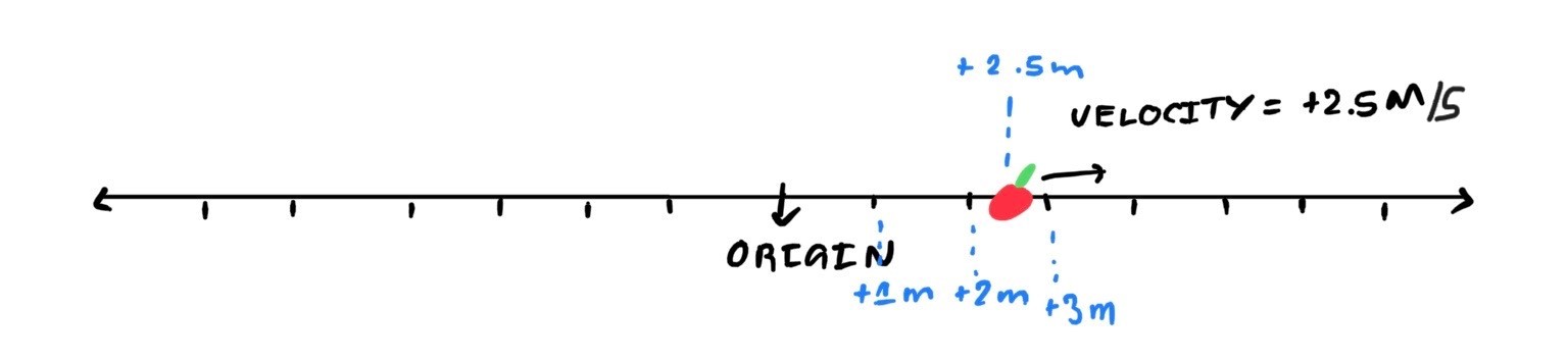
For example, if the apple is +10 metres from the origin, its velocity is +10 m/s (moving to the right). If the apple is at the origin, it does not move. If the apple is -12.5 meters from the origin, its velocity is -12.5 m/s (moving to the left).
Given some initial position of the apple, our task is to simulate the movement of the apple and to track its location every second. I ask the reader to take the following, very approximate proposition as granted.
If the apple is at a certain distance from the origin, a second later, its position is given by:
New Position = Current Position + Velocity
Thus we have all the ingredients to track the apple. Employing the algorithm devised in the previous section, we have:
- Analyse the system: There is no current state of the system. I introduce the initial condition that apple is at +2 meters travelling at +2 m/s.
- Calculate: Using the given equation, the position of the apple a second later is 2 + 2 = 4 meters. At +4 meters, it travels at +4 m/s via our one and only law of physics.
- Analyse the system: The apple is at +4 meters travelling at +4 m/s.
- Calculate : Using the given equation, the position of the apple a second later is 4 + 4 = 8 meters. At +8 meters, it travels at +8 m/s.
- Repeat.
| Time in seconds |
Position | Velocity |
| 0 | +2 m | +2 m/s |
| 1 | +4 m | +4 m/s |
| 2 | +8 m | +8 m/s |
| 3 | +16 m | +16 m/s |
This may be a spectacularly uneventful universe but nevertheless it perfectly captures the spirit of simulation.
V. Modelling Fluid Dynamics
Suffice to say, the physics on Europa involves a few more layers of complexity. In the scenario previously presented, we kept track of two variables: position and velocity. The system had just one equation controlling it.
In the case of Europa we must track velocity, salt concentration, temperature, pressure, and phase. Phase describes whether a specific location on our model is water or ice. The entire system is governed by the following equations:
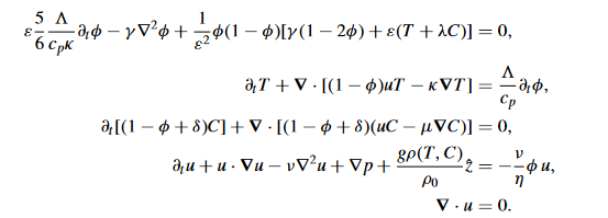
The equations may look rightfully daunting but can be explained very simply. From top-downwards: (1) controls the evolution of phase, that is, how the ice layer varies, (2) describes the evolution of temperature in the system, (3) controls the evolution of salt concentration in the fluid, (4) controls the movement of the fluid itself, (5) imposes the condition that density does not generally vary.
There may be more variables and equations at play, but the philosophy of simulation remains the same: analyse the current state, and then calculate the state a tiny bit into the future.
VI. Spectral Methods
For the maths-savvy folk I include a section on how our model "calculates the state a tiny bit into the future". If the reader is familiar with at least A-level mathematics, I invite them to read this section. Knowledge of linear algebra and Fourier transforms would also be useful.
Describing a five-equation coupled system is quite frankly beyond my paygrade, and thus I resort to simulating a wave on a one-dimensional string. The situation might be much simpler but the method remains the same.
The wave equation in one-dimension is given by:
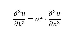
Where u is the wave amplitude, t is time, x is distance, and alpha is the wave speed. For this method, we assume that the solution to u is given as an infinite sum of orthogonal sinusoids.
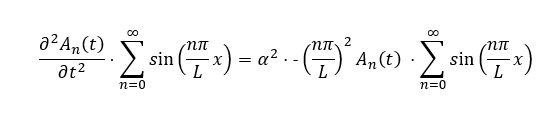
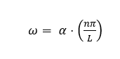
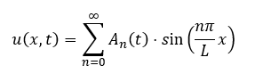 Where An are unique Fourier coefficients computed by performing a fast fourier transform (hence why spectral methods are incredibly fast). The length of the string is denoted by L. Substituting this expression back into the wave equation and simplifying, we get:
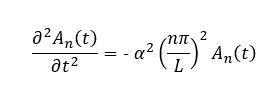
From observation, we can deduce that the solution to An is a complex exponential:
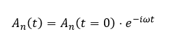
 Given a certain set of Fourier coefficients that describe the system, we can find the state of the system a tiny bit in the future via:
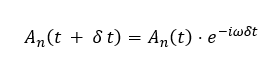
Since the Fourier coefficients effectively describe the system, knowing their future values allows us to completely understand its evolution.
Physics undergraduate at the University of St Andrews.


Please sign in
If you are a registered user on Laidlaw Scholars Network, please sign in